By Edit Gyenge | Jan 25, 2025
A fresh start—whether it’s a new year or just a new chapter in life—is the perfect time to build better habits. Maybe you want to exercise more, drink enough water, or finally get into the habit of reading every day. The key to success? Consistency. Small daily actions add up, and tracking your progress can make all the difference.
Sure, there are plenty of apps out there, but sometimes you just need a clear, visual way to see how you’re doing—month after month. That’s exactly why I created this Excel habit tracker! It’s the same one I use to keep myself accountable, and by the end of the year, you’ll have a snapshot of how your habits have evolved over time. Simple, flexible, and perfect for Excel fans.
Want to try it out? In this post, I’ll show you how to set up and customize your own habit tracker—so you can stay on top of your goals and actually see your progress. Let’s get started!
Create a Macro-Enabled Workbook
– Open a new or existing Excel file.
– Click File → Save As.
– Under Save as type, choose Excel Macro-Enabled Workbook (.xlsm) and save your file.
– Name the sheet “Data” (this is important for the next steps)
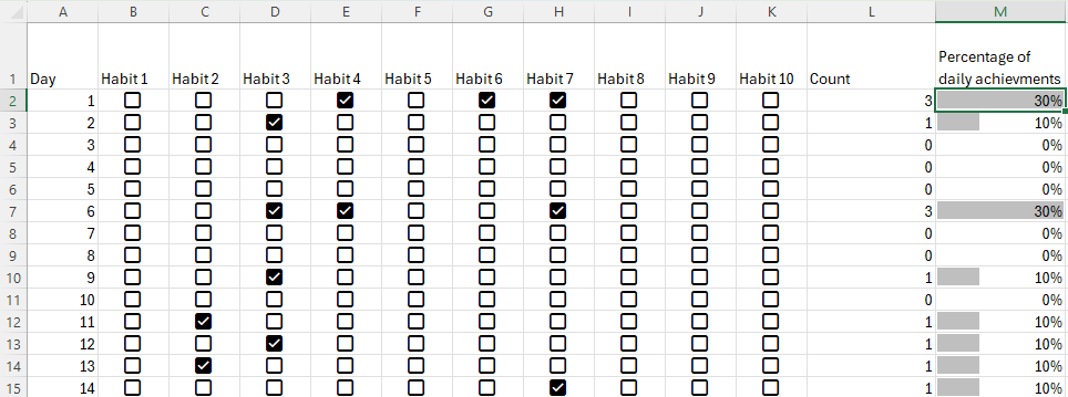
Prepare Your Data Worksheet
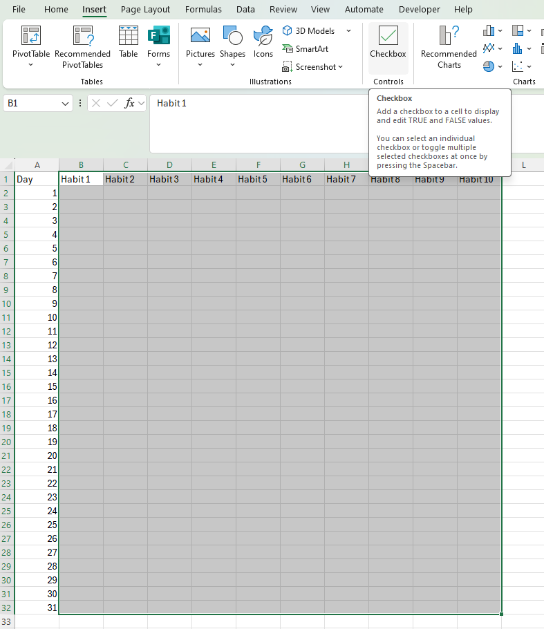
– In Column A, list day numbers (1, 2, 3, …, 31), depending on the month.
– In Columns B through K, set up labels for your 10 habits (e.g., “Habit 1,” “Habit 2,” etc.).
– Select the Habit coluns

You can format these cells as TRUE/FALSE by selecting your habit columns and go to Insert → Checkbox
Now, you’ll have a list of all your habits with the option to check them off as you complete them. To track your daily progress, you might also want to add a count column next to your habits. This will tell you how many habits you’ve completed each day using the formula: =COUNTIF(B2:K2, “TRUE”)
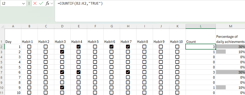
Next, you can add another column to track your daily progress percentage by using the formula: =L2/10
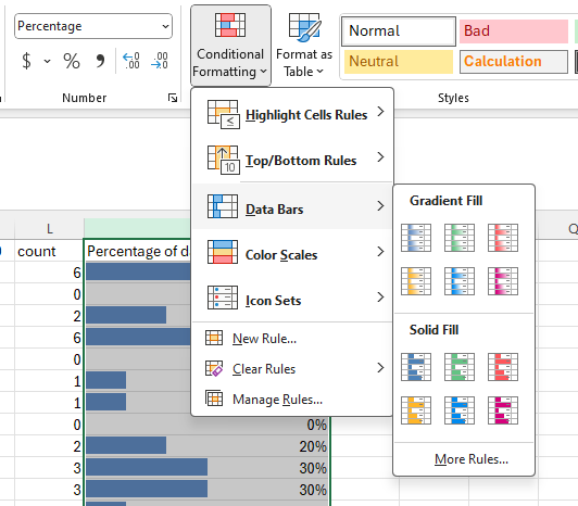
Then, format the column as a percentage and visualize it with a bar chart for an easy, at-a-glance view of your consistency.
Position Your Chart’s Center
– Decide where your radial chart will be centered. In this example, it’s around cell V20.
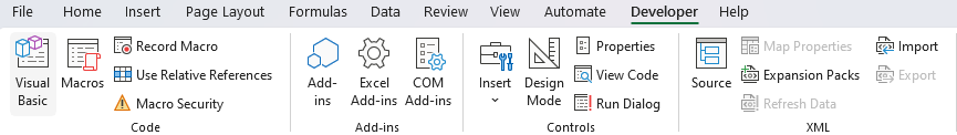
Open the VBA Editor
– Go to the Developer tab and click Visual Basic. (If you don’t see the Developer tab, you may need to enable it in your Excel options.)
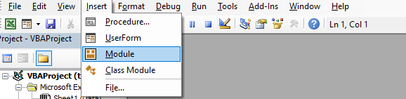
– In the VBA Editor, click Insert → Module to create a new blank module.
Add the VBA Code
– Copy and paste the provided code (see below) into your new module.
					Option Explicit

Sub CreateOrUpdateRadialShapes_WithDonutHole()
    '--- 1) Reference the Worksheet ---
    Dim ws As Worksheet
    Set ws = ThisWorkbook.Sheets("Data") ' <-- CHANGE if your sheet is named differently

    '--- 2) Identify the center cell (Y20) and compute center in points ---
    Dim rngCenter As Range
    Set rngCenter = ws.Range("Y20")  ' <-- This is your center cell

    Dim centerX As Single, centerY As Single

    ' Add a manual offset to shift left by about 3 columns:
    Dim shiftLeft As Single
    shiftLeft = 180  ' ~3 columns wide in points (adjust as needed)

    centerX = rngCenter.Left + (rngCenter.Width / 2) - shiftLeft
    centerY = rngCenter.Top + (rngCenter.Height / 2)

    '--- 3) Define day/habit counts ---
    Dim totalDays As Long: totalDays = 31
    Dim totalHabits As Long: totalHabits = 10

    '--- 4) Geometry parameters ---
    Dim angleStep As Double
    angleStep = 360# / totalDays

    Dim angleStepRad As Double
    angleStepRad = angleStep * WorksheetFunction.Pi() / 180#

    Dim donutHole As Single
    donutHole = 40    ' radius of the inner white circle

    Dim outerRadius As Single
    outerRadius = 200

    Dim radiusStep As Single
    radiusStep = (outerRadius - donutHole) / totalHabits

    ' If you want day 1 at the top, set startAngle = -90.
    Dim startAngle As Double
    startAngle = 0

    '--- 4b) Define a color for each habit ---
    Dim habitColors(1 To 10) As Long
    habitColors(1) = RGB(44, 209, 230)
    habitColors(2) = RGB(166, 209, 101)
    habitColors(3) = RGB(245, 173, 200)
    habitColors(4) = RGB(255, 177, 63)
    habitColors(5) = RGB(40, 77, 183)
    habitColors(6) = RGB(190, 173, 242)
    habitColors(7) = RGB(241, 224, 109)
    habitColors(8) = RGB(227, 113, 110)
    habitColors(9) = RGB(199, 181, 137)
    habitColors(10) = RGB(80, 159, 85)

    '--- 5) Loop through each day & habit ---
    Dim dayIdx As Long, habitIdx As Long
    For dayIdx = 1 To totalDays

        Dim angleDeg As Double
        angleDeg = startAngle + (dayIdx - 1) * angleStep

        Dim angleRad As Double
        angleRad = angleDeg * WorksheetFunction.Pi() / 180#

        For habitIdx = 1 To totalHabits

            ' 5b) The radial band for this habit
            Dim innerR As Single, outerR As Single
            innerR = donutHole + (habitIdx - 1) * radiusStep
            outerR = donutHole + habitIdx * radiusStep

            Dim midR As Single
            midR = (innerR + outerR) / 2

            ' 5c) Unique shape name
            Dim shpName As String
            shpName = "Day" & dayIdx & "_Habit" & habitIdx

            ' 5d) Check if shape exists
            Dim shp As Shape
            On Error Resume Next
            Set shp = ws.Shapes(shpName)
            On Error GoTo 0

            If shp Is Nothing Then
                Set shp = ws.Shapes.AddShape(msoShapeRectangle, 0, 0, 10, 10)
                shp.Name = shpName
            End If

            ' 5e) Size the shape
            Dim W As Single
            W = outerR - innerR

            Dim chord As Double
            chord = 2 * midR * Sin(angleStepRad / 2)

            shp.Width = W
            shp.Height = chord

            ' Outline styling
            shp.Line.Weight = 0.1
            shp.Line.ForeColor.RGB = RGB(197, 197, 197)
            ' or shp.Line.Visible = msoFalse to remove outline

            ' 5f) Position shape
            Dim shapeCenterX As Single, shapeCenterY As Single
            shapeCenterX = centerX + midR * Cos(angleRad)
            shapeCenterY = centerY + midR * Sin(angleRad)

            shp.Left = shapeCenterX - (W / 2)
            shp.Top = shapeCenterY - (chord / 2)

            ' 5h) Rotate to point outward
            shp.Rotation = angleDeg

            ' 5i) Color based on TRUE/FALSE
            Dim cellVal As Variant
            cellVal = ws.Cells(dayIdx, habitIdx + 1).Value

            If cellVal = True Then
                shp.Fill.ForeColor.RGB = habitColors(habitIdx)
            Else
                shp.Fill.ForeColor.RGB = RGB(239, 238, 235)
            End If

            Set shp = Nothing
        Next habitIdx
    Next dayIdx
End Sub
– Close or minimize the VBA editor to return to Excel.
Run the Macro
– In Excel, go back to the Developer tab and click Macros (or press Alt+F8).
– Select CreateOrUpdateRadialShapes from the list, then click Run.
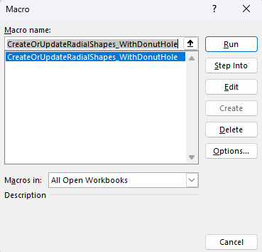
– Excel will generate 31×10 = 310 rectangular shapes around cell Y20, creating 31 radial “wedges,” each split into 10 segments.
Enable Automatic Recoloring
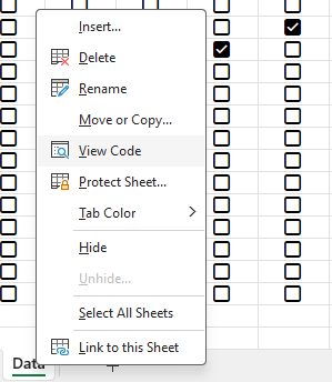
– To update colors automatically when you change any TRUE/FALSE values: right-click the “Data” sheet tab at the bottom of Excel and choose View Code. In the VBA editor window that appears, paste the additional code snippet provided.
					Private Sub Worksheet_Change(ByVal Target As Range)
    On Error GoTo Cleanup

    ' Optional: If your TRUE/FALSE values live in a specific range (e.g., B1:K31)
    ' we can check if the changed cell intersects that range:
    If Not Intersect(Target, Me.Range("B1:K31")) Is Nothing Then

        ' Temporarily disable events to avoid recursion
        Application.EnableEvents = False

        ' Call your macro. Replace with your actual macro name:
        Call CreateOrUpdateRadialShapes_WithDonutHole
    End If

Cleanup:
    ' Re-enable events
    Application.EnableEvents = True
End Sub
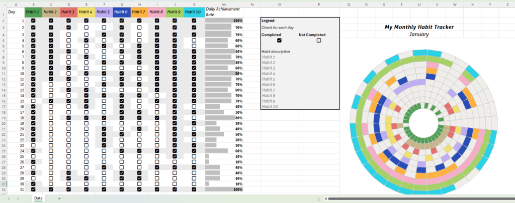
And that’s it! Of course, you can customize the colors to match your style. I love using Coolors.co to find palettes that make my charts both functional and visually appealing. A well-designed chart can be surprisingly motivating, so feel free to experiment with different looks!
I also added legends and some visual tweaks to keep everything clear and easy to read. Here’s the final result!

The best part? You can adapt this setup for anything—not just habit tracking. Use it for KPIs, goal tracking, or any data you want to visualize. The key is to create a simple, engaging way to track what matters to you, so you stay motivated and see your progress at a glance!
Check out some of my latest

